00 - Setup

import os
import stampede as st
import pandas as pd
import scanpy as sc
import matplotlib.pyplot as plt

from pydeseq2.ds import DeseqStats
from pydeseq2.dds import DeseqDataSet

# dictionary with input files per slide
slides = {
    1: {
        "exprmat": "exprMat_file.csv.gz",
        "metadata": "metadata_file.csv.gz",
        "fov_positions": "fov_positions_file.csv.gz",
    }
}
# optional filepath prefix
data_dir = "data"

os.makedirs(st.config["adata_dir"], exist_ok=True)

01 - Read

# table mapping the FOVs per slide to each sample
# column "fovs" accepts any combination of comma separated values (e.g. 1,2,3) and ranges (e.g. 4-6)
samples_df = pd.read_table("data/sample2fov.csv", sep=",")
st.validate_input(slides, samples_df, data_dir)
samples_df

	sample	fovs	slide
0	s1	10-18	1
1	s2	19-27	1
2	s3	28-36	1

# combine the input files into a single cell object and write it to file
adata_file = os.path.join(st.config["adata_dir"], "raw_data.h5ad")
st.read_cosmx(
    slides,
    samples_df,
    adata_file,
    data_dir=data_dir,
    overwrite=False,
    verbose=True,
)

adata_file already exists and overwrite=False

'adatas/raw_data.h5ad'

adata = sc.read_h5ad(adata_file)
adata.obs

	fov	cell_ID	slide	slide-fov	Area	AspectRatio	CenterX_local_px	CenterY_local_px	Width	Height	...	nCount	nCountPerCell	nFeaturePerCell	propNegativeCellAvg	complexityCellAvg	errorCtPerCellEstimate	percOfDataFromErrorPerCell	qcFlagsFOV	sample	fovs
slide-fov-cell_ID
1-10-1	10	1	1	1-10	4260	0.97	2902	613	77	75	...	140803	863.822086	670.730061	0.000315	1.245668	87.131902	0.100868	Pass	s1	10-18
1-10-2	10	2	1	1-10	5228	0.95	3007	623	83	87	...	140803	863.822086	670.730061	0.000315	1.245668	87.131902	0.100868	Pass	s1	10-18
1-10-3	10	3	1	1-10	3204	0.89	2947	649	71	63	...	140803	863.822086	670.730061	0.000315	1.245668	87.131902	0.100868	Pass	s1	10-18
1-10-4	10	4	1	1-10	22940	0.81	2833	746	191	237	...	140803	863.822086	670.730061	0.000315	1.245668	87.131902	0.100868	Pass	s1	10-18
1-10-5	10	5	1	1-10	4404	0.76	2990	691	93	71	...	140803	863.822086	670.730061	0.000315	1.245668	87.131902	0.100868	Pass	s1	10-18
...	...	...	...	...	...	...	...	...	...	...	...	...	...	...	...	...	...	...	...	...	...
1-36-271	36	271	1	1-36	4264	0.88	1812	2281	81	71	...	110510	401.854545	338.160000	0.000438	1.168196	46.031818	0.114548	Pass	s3	28-36
1-36-272	36	272	1	1-36	5024	0.79	397	3328	87	69	...	110510	401.854545	338.160000	0.000438	1.168196	46.031818	0.114548	Pass	s3	28-36
1-36-273	36	273	1	1-36	5460	0.98	323	3370	83	81	...	110510	401.854545	338.160000	0.000438	1.168196	46.031818	0.114548	Pass	s3	28-36
1-36-274	36	274	1	1-36	1888	0.96	455	3372	47	49	...	110510	401.854545	338.160000	0.000438	1.168196	46.031818	0.114548	Pass	s3	28-36
1-36-275	36	275	1	1-36	3880	0.97	398	3397	69	67	...	110510	401.854545	338.160000	0.000438	1.168196	46.031818	0.114548	Pass	s3	28-36

27625 rows × 79 columns

02 - QC

02a - Slide QC

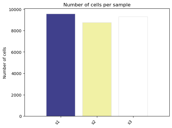
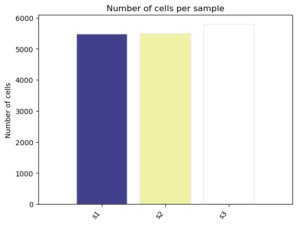
fig, ax = st.pl.ncell_per_condition(adata, "sample")
plt.show()

st.pp.slide_qc(adata, slides, ["sample"], data_dir=data_dir)
adata.uns["fov_metadata"].head()

	slide	fov	x	y	nCounts	nCell	mean_CountsPerCell	nCount_negprobes	mean_NegProbe-CountsPerCell	nCount_falsecode	mean_FalseCode-CountsPerCell	mean_CellSize	sample
slide-fov
1-10	1	10	19773	149405	140803	163	863.822086	46	0.282209	480	2.944785	63.957736	s1
1-11	1	11	24029	149405	752088	848	886.896226	274	0.323113	2569	3.029481	54.344592	s1
1-12	1	12	28285	149405	50213	47	1068.361702	21	0.446809	151	3.212766	74.681880	s1
1-13	1	13	19773	145149	1241593	1866	665.376742	521	0.279207	5842	3.130761	52.223075	s1
1-14	1	14	24029	145149	2638265	3391	778.019758	916	0.270127	10325	3.044825	52.564838	s1

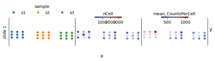
# this dataset was subset from a much larger slide
# the plot limits in this tutorial are extended to provide a sense of scale
fig, axs = st.pl.slide_qc(
    adata, columns=["sample", "nCell", "mean_CountsPerCell"], figsize=(2.5, 0.5), legend_kwargs={"ncols": 3}
)
ylim = axs[1, 0].get_ylim()
axs[1, 0].set_ylim(ylim[0]-10_000, ylim[1]+20_000)
plt.show()

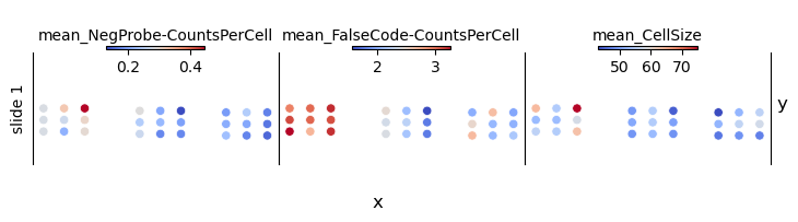
fig, axs = st.pl.slide_qc(
    adata, columns=["mean_NegProbe-CountsPerCell", "mean_FalseCode-CountsPerCell", "mean_CellSize"], figsize=(2.5, 0.5)
)
ylim = axs[1, 0].get_ylim()
axs[1, 0].set_ylim(ylim[0]-10_000, ylim[1]+20_000)
plt.show()

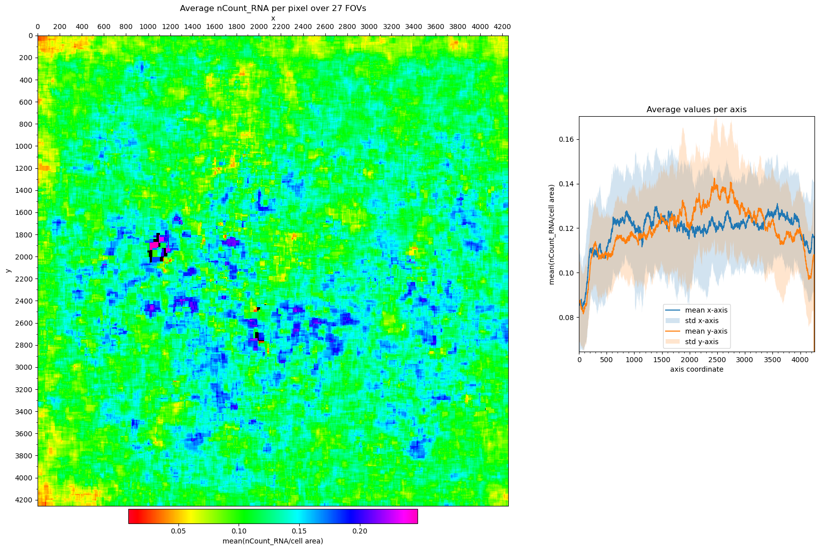
Visualizing Field of View edge-effects

Cells on the edges of an Field of View (FOV) may have been truncated. Furthermore, we tend to detect less RNA in them. There may also be a bias to the corners and/or one or two edges in the dataset.

# plot the average nCount_RNA per pixel over all FOVs
fig, axs = st.pl.avg_per_pixel(
    adata, column='nCount_RNA', normalize_cell_area=True
)
plt.show()

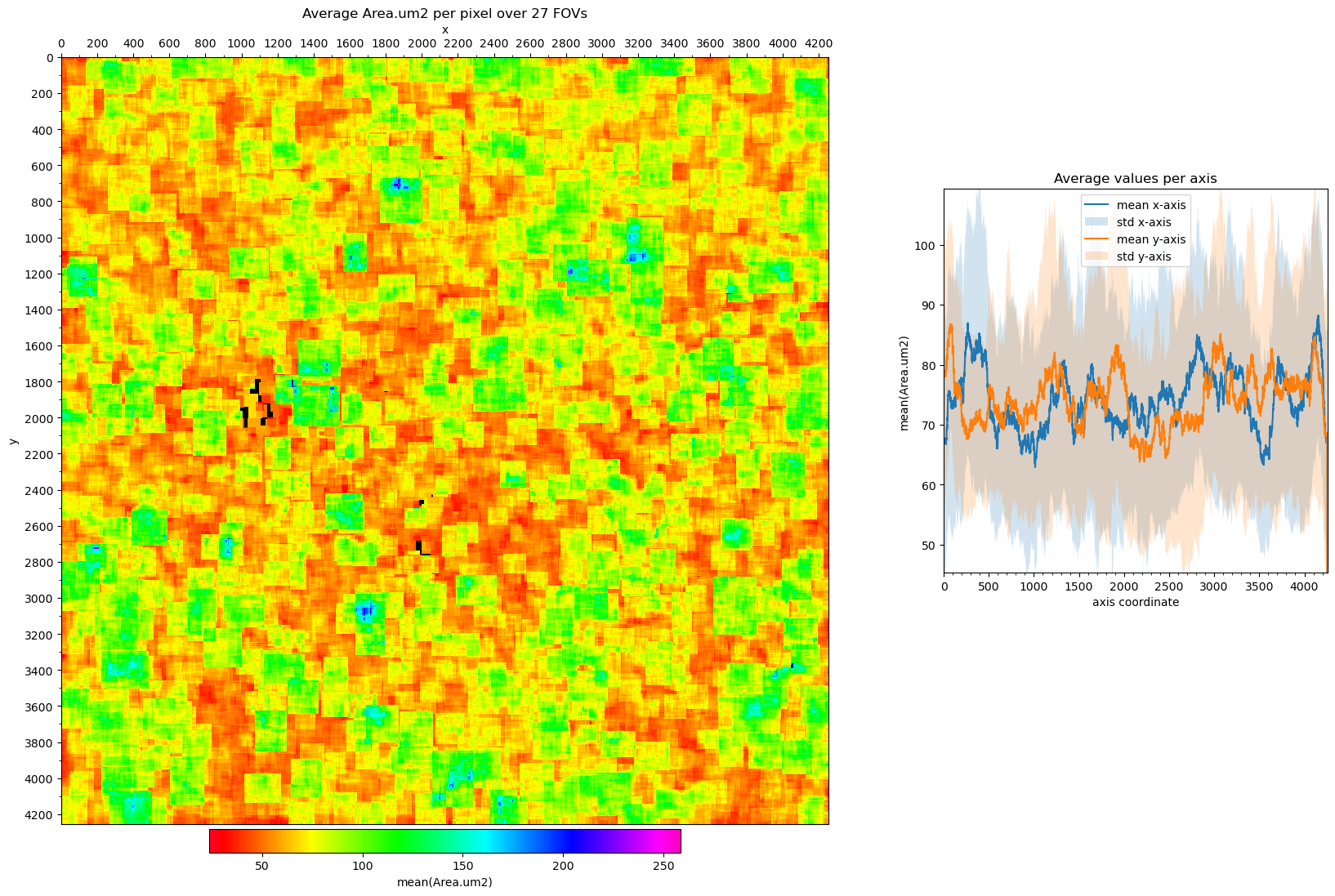
# plot the cell area for all FOVs. 
# (do not normalize for cell area when plotting the cell area)
fig, axs = st.pl.avg_per_pixel(
    adata, column='Area.um2', normalize_cell_area=False
)
plt.show()

# visualize the effect of removing cells based on distance to FOV edge
fig, axs = st.pl.correlations(adata, xcolumn="dist2edge_px", ycolumn="nCount_RNA", max_quantile=0.7)

dist2edge_threshold = 50
print(f"{dist2edge_threshold=}")
axs[1, 1].axvline(dist2edge_threshold, color="red")
plt.show()

dist2edge_threshold=50

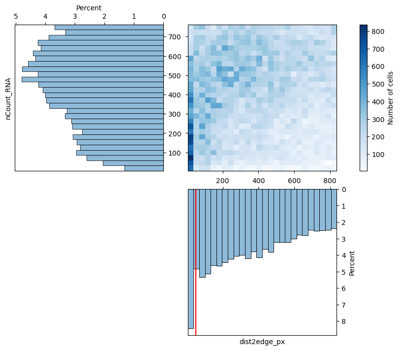
adata = st.pp.filter_edges(adata, dist2edge_threshold)

1_729 cells filtered out, 25_896 cell remaining.

02b - gene QC

# remove non-PBMC genes
fname = os.path.join(data_dir, "blacklist_pbmc_6k.txt")
blacklist = pd.read_table(fname, header=None)[0].to_list()

before = len(adata.var)
adata = adata[:, ~adata.var.index.isin(blacklist)].copy()
after = len(adata.var)
print(before - after, "genes filtered out")

904 genes filtered out

# mark core immune genes
fname = os.path.join(data_dir, "core_immune_genes_6k.txt")
whitelist = pd.read_table(fname, header=None)[0].to_list()
adata.var["is_core_immune_gene"] = adata.var.index.isin(whitelist)

# determine a noise threshold for gene expression using the mean expression 
# and standard deviation of the negative control probes
st.pp.gene_qc(adata)
adata.var

	is_core_immune_gene	is_negctrl	is_sysctrl	nCell	pctCell	nTranscript	mean_Transcript	above_noise
A1BG	False	False	False	5625	21.721501	6883	0.265794	True
A2M	True	False	False	635	2.452116	658	0.025409	True
AAAS	False	False	False	1416	5.468026	1496	0.057770	True
AAK1	True	False	False	2175	8.398981	2363	0.091250	True
AAMP	False	False	False	1483	5.726753	1591	0.061438	True
...	...	...	...	...	...	...	...	...
ZSWIM6	True	False	False	854	3.297807	888	0.034291	True
ZWINT	True	False	False	969	3.741891	1019	0.039350	True
ZYG11B	False	False	False	1855	7.163268	2002	0.077309	True
ZYX	True	False	False	2650	10.233241	3012	0.116311	True
ZZZ3	True	False	False	1606	6.201730	1709	0.065995	True

5614 rows × 8 columns

fig, ax = st.pl.noise_threshold(adata, max_quantile=0.95)
plt.show()

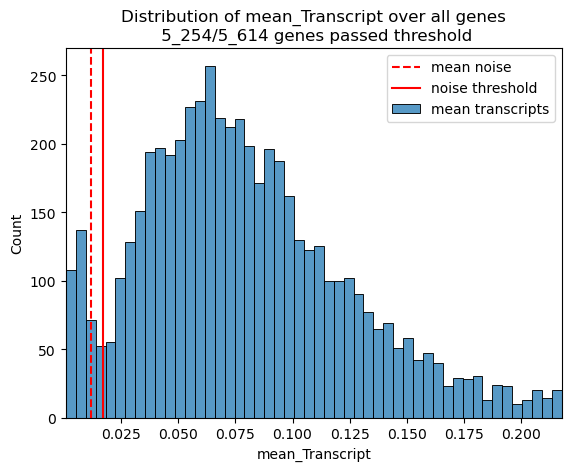
adata = st.pp.filter_genes(adata)

377 genes filtered out, 5_237 genes remaining.

02c - cell QC

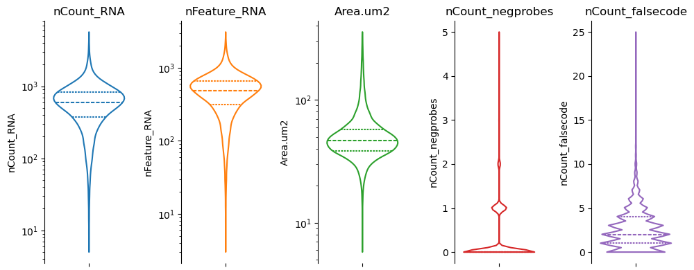
fig, axs = st.pl.violin(
    adata, 
    ["nCount_RNA", "nFeature_RNA", "Area.um2", "nCount_negprobes", "nCount_falsecode"],
    log_scale=(True, True, True, False, False)
)
plt.show()

adata = st.pp.filter_cells(
    adata, 
    falsecode_max = 5,
    negprobe_max = 2,
    ntranscript_min = 250,
    ntranscript_max = 1500,
    area_min = 25,
    area_max = 110,
)

9_123 cells filtered out, 16_773 cells remaining.

st.pp.gene_qc_postfilter(adata)
adata.var[["nCell", "nCell_postfilter", "pctCell", "pctCell_postfilter"]]

	nCell	nCell_postfilter	pctCell	pctCell_postfilter
A1BG	5625	3674	21.721501	21.90
A2M	635	417	2.452116	2.49
AAAS	1416	952	5.468026	5.68
AAK1	2175	1434	8.398981	8.55
AAMP	1483	922	5.726753	5.50
...	...	...	...	...
ZSWIM6	854	547	3.297807	3.26
ZWINT	969	605	3.741891	3.61
ZYG11B	1855	1180	7.163268	7.04
ZYX	2650	1766	10.233241	10.53
ZZZ3	1606	1067	6.201730	6.36

5237 rows × 4 columns

st.pp.cell_qc_postfilter(adata)
adata.obs[["nFeature_RNA", "nFeature_RNA_postfilter", "nCount_RNA", "nCount_RNA_postfilter"]]

	nFeature_RNA	nFeature_RNA_postfilter	nCount_RNA	nCount_RNA_postfilter
slide-fov-cell_ID
1-10-1	627	560	821	748
1-10-2	873	771	1185	1067
1-10-6	648	573	838	748
1-10-8	831	716	1015	888
1-10-9	666	583	823	730
...	...	...	...	...
1-36-269	750	643	900	786
1-36-270	725	629	863	754
1-36-272	847	718	1033	894
1-36-273	814	711	989	871
1-36-275	660	562	782	676

16773 rows × 4 columns

fig, ax = st.pl.ncell_per_condition(adata, columns = ["sample"])
plt.show()

03 - Dimensionality reduction

st.pp.binarize(adata)

binary layer set as adata.X

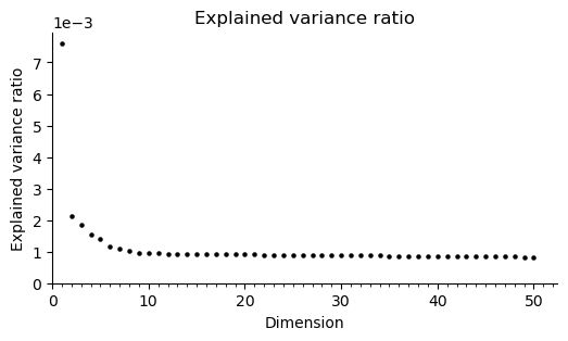
st.pp.dim_red(adata, use_genes="is_core_immune_gene")
fig, ax = st.pl.scree(adata)
plt.show()

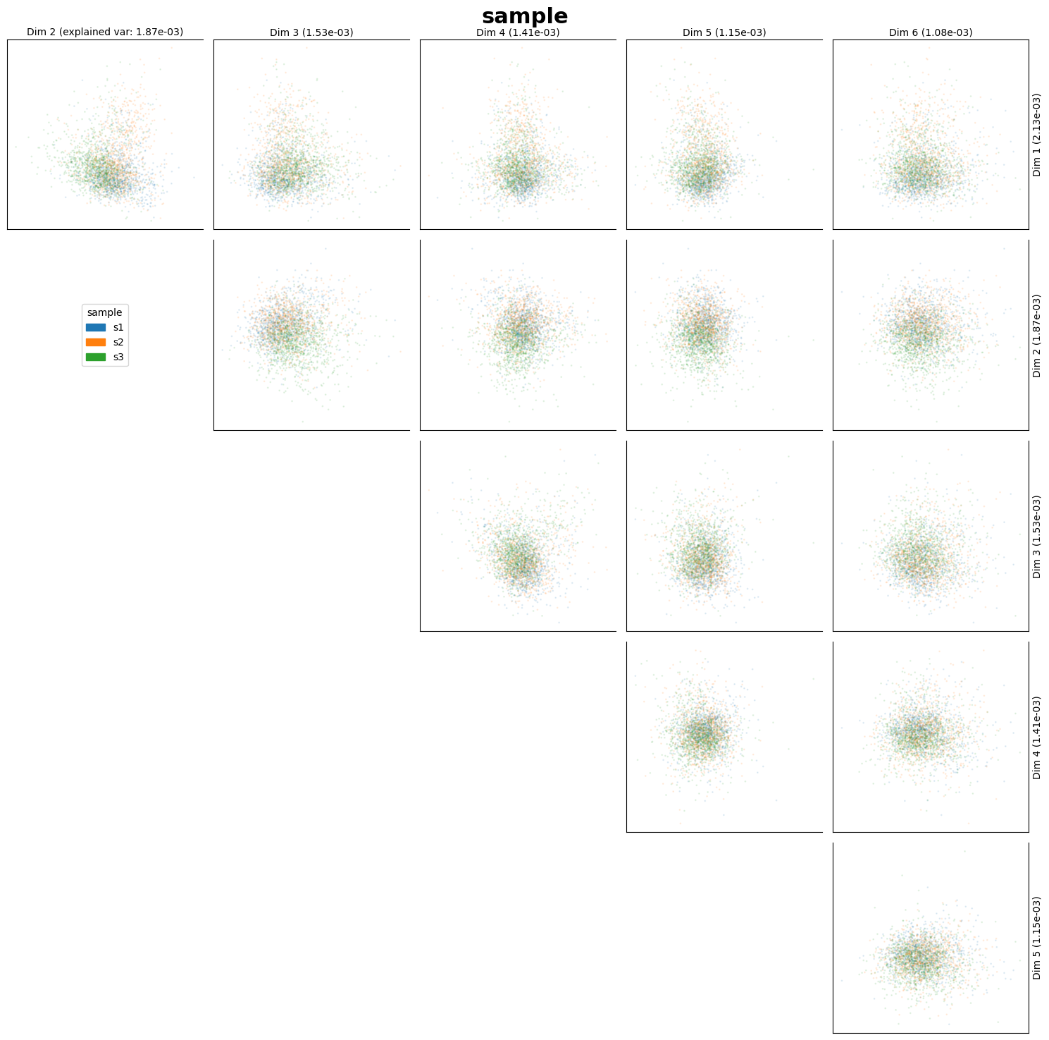
fig_ax_list = st.pl.dim_red(
    adata, 
    columns=["sample"],
    subset_size=1000,
)
plt.show()

sc.pp.neighbors(
    adata,
    use_rep="X_svd",
    key_added="neighbors_svd",
)

sc.tl.umap(
    adata,
    neighbors_key="neighbors_svd",
    key_added="umap_svd",
)

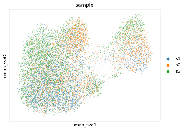
sc.pl.embedding(
    adata,
    basis="umap_svd",
    color="sample",
    alpha=0.5,
)

04 - Clustering

st.pp.knn_count_smoothing(
    adata,
    neighbors_key="neighbors_svd",
)

KNN_binary_mean layer set as adata.X

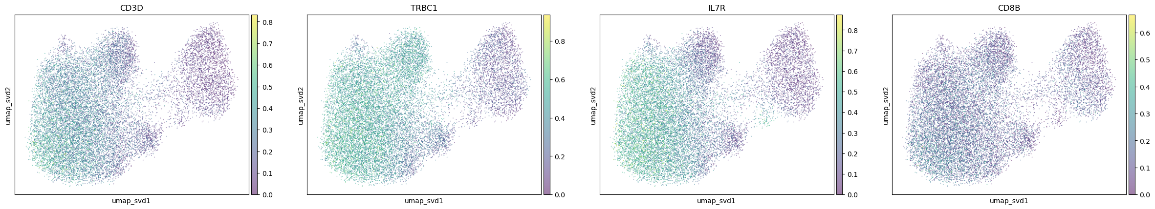
markerdict = {
    "T_cells": [
        "CD3D", "TRBC1","IL7R", "CD8B",
    ],
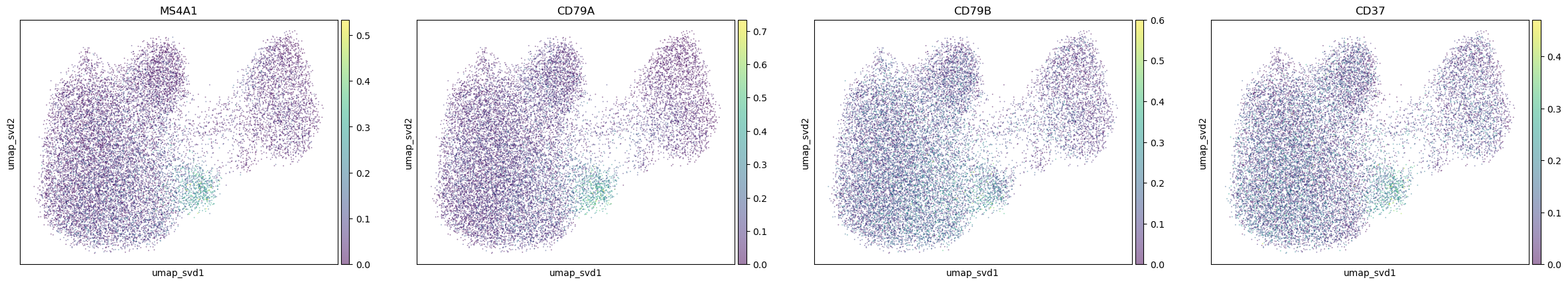
    "B_cells": [
        "MS4A1", "CD79A", "CD79B", "CD37"
    ],
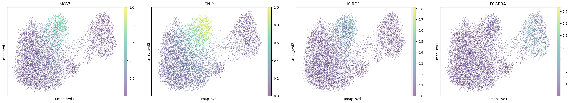
    "NK_cells": [
        "NKG7", "GNLY", "KLRD1", "FCGR3A"
    ],
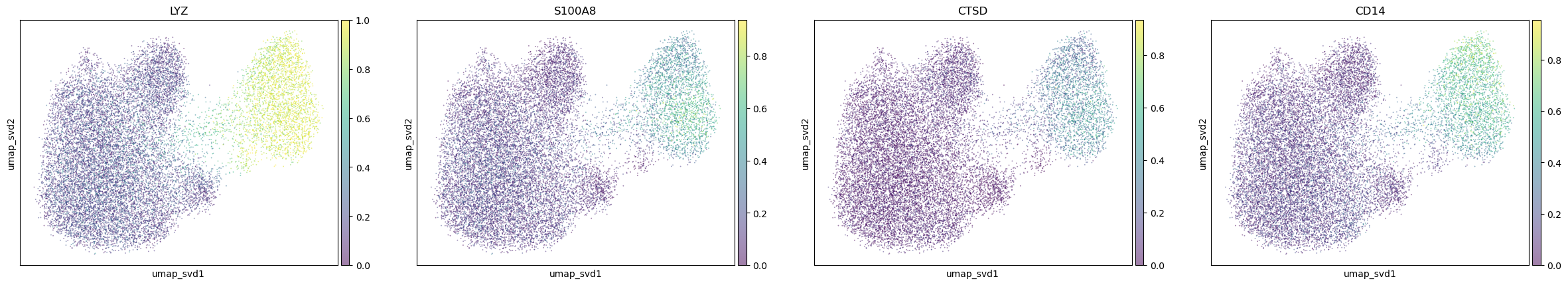
    "Monocytes_Macrophages": [
        "LYZ", "S100A8", "CTSD", "CD14",
    ],
}

for ctype, markers in markerdict.items():
    print(ctype)
    sc.pl.embedding(
        adata,
        basis="umap_svd",
        color=markers,
        layer="KNN_binary_mean",
        ncols=4,
        alpha=0.5,
    )

T_cells

B_cells

NK_cells

Monocytes_Macrophages

res = 0.5
sc.tl.leiden(
    adata,
    resolution=res,
    neighbors_key="neighbors_svd",
    key_added=f"leiden_res_{res:.2f}",
    flavor="igraph",
    n_iterations=2,
    directed=False,
    random_state=42,
)

sc.tl.rank_genes_groups(adata, f"leiden_res_{res:.2f}", n_genes=6, layer="binary")
sc.tl.dendrogram(adata, f"leiden_res_{res:.2f}", use_rep="X_svd")
sc.pl.rank_genes_groups_matrixplot(
    adata,
    n_genes=6,
)

WARNING: It seems you use rank_genes_groups on the raw count data. Please logarithmize your data before calling rank_genes_groups.

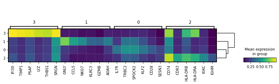
cluster2ctype = {
    "0": "T_cells",
    "1": "NK_cells",
    "2": "B_cells",
    "3": "Myeloid_cells",
}
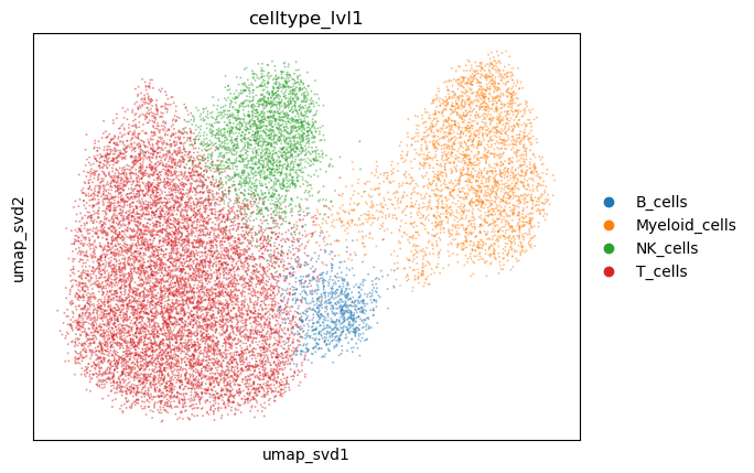
adata.obs["celltype_lvl1"] = adata.obs[f"leiden_res_{res:.2f}"].astype(str).replace(cluster2ctype).astype("category")

sc.pl.embedding(
    adata,
    basis="umap_svd",
    color="celltype_lvl1",
    alpha=0.5,
)

05 - Differential expression analysis

st.pp.combine_obs_columns(adata, ["sample", "celltype_lvl1"], "sample_celltype")
adata.obs["sample_celltype"].value_counts().head()

sample_celltype
s1_T_cells          4003
s3_T_cells          3912
s2_T_cells          2483
s2_NK_cells         1359
s2_Myeloid_cells    1351
Name: count, dtype: int64

05a - using detection rates & pbGLM

det_rate_df = st.pp.detection_rates(adata, "sample_celltype")
det_rate_df

	s1_T_cells	s3_T_cells	s2_T_cells	s2_NK_cells	s2_Myeloid_cells	s3_Myeloid_cells	s1_Myeloid_cells	s3_NK_cells	s1_NK_cells	s3_B_cells	s2_B_cells	s1_B_cells
A1BG	0.166938	0.186624	0.192226	0.180092	0.241642	0.234460	0.198680	0.152472	0.154464	0.222320	0.177528	0.168530
A2M	0.022996	0.016689	0.019951	0.024067	0.019234	0.015267	0.023463	0.016206	0.023768	0.027226	0.022711	0.013955
AAAS	0.046860	0.046575	0.053780	0.039238	0.046576	0.037077	0.039669	0.037278	0.053029	0.051782	0.071536	0.051186
AAK1	0.076153	0.075050	0.077622	0.067599	0.053272	0.056707	0.068781	0.092419	0.077461	0.051782	0.042722	0.019593
AAMP	0.044045	0.040120	0.048625	0.032338	0.047914	0.047983	0.065840	0.038899	0.047833	0.049051	0.071536	0.059978
...	...	...	...	...	...	...	...	...	...	...	...	...
ZSWIM6	0.026101	0.020126	0.022668	0.024756	0.045907	0.041439	0.040629	0.021068	0.022061	0.027226	0.017018	0.030966
ZWINT	0.032164	0.033675	0.026749	0.031648	0.018569	0.032715	0.025359	0.019447	0.032328	0.032678	0.028416	0.019593
ZYG11B	0.061227	0.052116	0.061703	0.058594	0.064679	0.061069	0.054143	0.056735	0.056500	0.057245	0.071536	0.028111
ZYX	0.064447	0.086215	0.068612	0.069678	0.139921	0.201745	0.144557	0.113513	0.068700	0.076388	0.048464	0.068847
ZZZ3	0.050390	0.053733	0.058255	0.052366	0.044569	0.050164	0.055113	0.058357	0.046104	0.068180	0.062864	0.036702

5237 rows × 12 columns

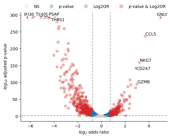
%%time
results_df1 = st.tl.paired_binomial_glm(
    det_rate_df, 
    adata, 
    column="sample_celltype", 
    test_condition="NK_cells", 
    reference_condition="Myeloid_cells", 
    condition_column="celltype_lvl1",
)
results_df1

CPU times: user 22.3 s, sys: 15.9 ms, total: 22.3 s
Wall time: 22.3 s

	beta	se	odds_ratio	pval	perfect_separation	error	padj	-log10(padj)	log2(odds_ratio)
gene
IFI30	-4.339651	0.090796	0.013041	0.000000e+00	False	None	0.000000e+00	9.0	-6.260793
TIMP1	-4.036057	0.084280	0.017667	0.000000e+00	False	None	0.000000e+00	9.0	-5.822799
LYZ	-3.551084	0.079467	0.028694	0.000000e+00	False	None	0.000000e+00	9.0	-5.123131
PSAP	-3.309378	0.073933	0.036539	0.000000e+00	False	None	0.000000e+00	9.0	-4.774423
THBS1	-3.108490	0.072474	0.044668	0.000000e+00	False	None	0.000000e+00	9.0	-4.484603
...	...	...	...	...	...	...	...	...	...
CD247	2.019324	0.078699	7.533233	3.378460e-145	False	None	5.529061e-143	9.0	2.913269
GZMB	2.077770	0.099078	7.986641	1.206773e-97	False	None	1.128548e-95	9.0	2.997589
NKG7	2.233148	0.082191	9.329190	1.460050e-162	False	None	3.058512e-160	9.0	3.221752
CCL5	2.563929	0.077387	12.986745	1.047344e-240	False	None	3.917816e-238	9.0	3.698968
GNLY	3.470331	0.078625	32.147383	0.000000e+00	False	None	0.000000e+00	9.0	5.006629

5237 rows × 9 columns

fig, ax = st.pl.paired_binomial_glm_volcano(results_df1)
plt.show()

05b - using pyDESeq2

counts = st.pp.pseudobulk(adata, "sample_celltype") 
counts

	s1_T_cells	s1_Myeloid_cells	s1_NK_cells	s1_B_cells	s2_T_cells	s2_Myeloid_cells	s2_NK_cells	s2_B_cells	s3_T_cells	s3_B_cells	s3_Myeloid_cells	s3_NK_cells
A1BG	917	198	88	56	550	355	259	61	800	81	215	94
A2M	135	25	14	5	59	29	35	8	73	10	14	10
AAAS	272	42	31	18	158	70	57	25	203	19	34	23
AAK1	436	72	45	7	227	80	98	15	326	19	52	57
AAMP	256	69	28	21	143	72	47	25	175	18	44	24
...	...	...	...	...	...	...	...	...	...	...	...	...
ZSWIM6	153	43	13	11	67	69	36	6	88	10	38	13
ZWINT	188	27	19	7	79	28	46	10	147	12	30	12
ZYG11B	353	57	33	10	181	97	85	25	227	21	56	35
ZYX	371	147	40	24	201	208	101	17	374	28	185	70
ZZZ3	292	58	27	13	171	67	76	22	234	25	46	36

5237 rows × 12 columns

%%time
results_df2 = st.tl.pydeseq2(
    counts, 
    adata, 
    column="sample_celltype", 
    test_condition="NK_cells", 
    reference_condition="Myeloid_cells", 
    condition_column="celltype_lvl1",
)
results_df2

Using None as control genes, passed at DeseqDataSet initialization

Fitting size factors...
... done in 0.00 seconds.

Fitting dispersions...
... done in 0.51 seconds.

Fitting dispersion trend curve...
/home/siebrenf/miniconda3/envs/stampede/lib/python3.14/site-packages/pydeseq2/dds.py:822: UserWarning: The dispersion trend curve fitting did not converge. Switching to a mean-based dispersion trend.
  self._fit_parametric_dispersion_trend(vst)
... done in 0.11 seconds.

Fitting MAP dispersions...
... done in 0.51 seconds.

Fitting LFCs...
... done in 0.51 seconds.

Calculating cook's distance...
... done in 0.01 seconds.

Replacing 0 outlier genes.

Running Wald tests...

Log2 fold change & Wald test p-value: celltype_lvl1 NK_cells vs Myeloid_cells
          baseMean  log2FoldChange     lfcSE      stat    pvalue      padj
A1BG    200.158056       -0.439831  0.150883 -2.915053  0.003556  0.021761
A2M      22.222461        0.166992  0.297768  0.560814  0.574924  0.787363
AAAS     51.730993        0.011885  0.219241  0.054211  0.956767  0.982888
AAK1     68.129857        0.377736  0.189506  1.993267  0.046232  0.170509
AAMP     53.521286       -0.496203  0.227030 -2.185632  0.028843  0.120262
...            ...             ...       ...       ...       ...       ...
ZSWIM6   30.811360       -0.894070  0.255361 -3.501200  0.000463  0.003743
ZWINT    30.131072        0.201892  0.270985  0.745032  0.456252  0.698725
ZYG11B   61.445199       -0.070701  0.197421 -0.358122  0.720252  0.875431
ZYX     103.154574       -0.952321  0.226699 -4.200818  0.000027  0.000275
ZZZ3     57.277142        0.076049  0.202864  0.374878  0.707751  0.869661

[5237 rows x 6 columns]
CPU times: user 3.09 s, sys: 120 ms, total: 3.21 s
Wall time: 4.09 s

... done in 0.46 seconds.

	baseMean	log2FoldChange	lfcSE	stat	pvalue	padj
A1BG	200.158056	-0.439831	0.150883	-2.915053	0.003556	0.021761
A2M	22.222461	0.166992	0.297768	0.560814	0.574924	0.787363
AAAS	51.730993	0.011885	0.219241	0.054211	0.956767	0.982888
AAK1	68.129857	0.377736	0.189506	1.993267	0.046232	0.170509
AAMP	53.521286	-0.496203	0.227030	-2.185632	0.028843	0.120262
...	...	...	...	...	...	...
ZSWIM6	30.811360	-0.894070	0.255361	-3.501200	0.000463	0.003743
ZWINT	30.131072	0.201892	0.270985	0.745032	0.456252	0.698725
ZYG11B	61.445199	-0.070701	0.197421	-0.358122	0.720252	0.875431
ZYX	103.154574	-0.952321	0.226699	-4.200818	0.000027	0.000275
ZZZ3	57.277142	0.076049	0.202864	0.374878	0.707751	0.869661

5237 rows × 6 columns

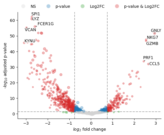
fig, axs = st.pl.pydeseq2_volcano(results_df2)
plt.show()